Lets do a quick exploration into some interesting properties of the fibonacci sequence!
Converting distances between miles and kilometers is something we’ve all done a bunch of times (maybe?). For as long as I can remember I’ve held the rough rule in my head of multiplying miles by 1.6 to get the rough amount of kilometers. This is perfectly acceptable. In 99% of day to day, this will be all you need.
However, I stumbled across a snippet recently that claimed something I found fascinating. Apparently you can use the fibonacci sequence to get a close approximation of a miles to kms conversion. Apparently if you take any fibonacci number (say, 5) and treat this as miles, then the next fibonacci will be an approximate conversion of the miles number into kilometers. 5 is followed by 8 in the fibonacci sequence. 5 * 1.6 = 8. Hmmm. Well that singular data point certainly supports the hypothesis! Lets dive into this in a data driven way and see how well this holds across a wide range of fibonacci numbers.
We’ll start by loading a few useful packages.
library(dplyr)
library(ggplot2)
library(tidyr)
library(ggforce)
In case you’re not aware, the Fibonacci sequence is a series of numbers where each number is the sum of the two preceding ones, starting from 0 and 1. So, the sequence begins 0, 1, 1, 2, 3, 5, 8, 13, and so on. It’s found in many natural patterns, from the arrangement of leaves on a stem to the spirals of shells, and has fascinating mathematical properties that make it useful in various fields, including computing, finance, and even conversion problems like the one we’ll explore here!
R does not come with a built in function that calculates the fibonacci sequence. It’s always useful to get some practise at writing functions, so this provides a good excuse.
my_fib <- function(n) {

  fib_vec <- numeric(n)

  fib_vec[1] <- 0
  if (n > 1) {
    fib_vec[2] <- 1
  }

  for (i in 3:n) {
    fib_vec[i] <- fib_vec[i - 1] + fib_vec[i - 2]
  }

  return(fib_vec)
}
Notice one important trick here - I preallocate the vector using numeric(n). This avoids growing the vector each time we add more data which is notoriously slow in R.
Lets do some quick spot checks of our function to check it looks correct.
my_fib(3)## [1] 0 1 1my_fib(6)## [1] 0 1 1 2 3 5my_fib(10)## [1] 0 1 1 2 3 5 8 13 21 34Seems to be correct! Note that this function does have some major issues - namely that it doesn’t handle values of 1 or 2, and that it has no checking for the input type. For example, these all fail (and the last one fails with a rather unhelpful error message).
my_fib(1)## Error in fib_vec[i] <- fib_vec[i - 1] + fib_vec[i - 2]: replacement has length zeromy_fib(2)## Error in fib_vec[i] <- fib_vec[i - 1] + fib_vec[i - 2]: replacement has length zeromy_fib("seven")## Warning in numeric(n): NAs introduced by coercion## Error in numeric(n): vector size cannot be NA/NaNLets quickly improve our function with some basic best practises. I also spotted something here - since we’re going to be comparing fibonacci numbers to the ones immediately following them, we don’t actually need to worry about the first two (which are 1 and 0). The first comparison we actually do is the 1 to 2, meaning we can actually ignore the first two values.
my_fib <- function(n) {

  if (!is.numeric(n) || n != as.integer(n) || n <= 0) {
    stop("Input must be a positive integer.", call. = FALSE)
  }

  fib_vec <- numeric(n)

  fib1 <- 1
  fib2 <- 2

  if(n == 1){
    fib_vec[1] <- fib1
  } else if(n == 2) {
    fib_vec[1] <- fib1
    fib_vec[2] <- fib2
  } else {
    fib_vec[1] <- fib1
    fib_vec[2] <- fib2

    for (i in 3:n) {
      fib_vec[i] <- fib_vec[i - 1] + fib_vec[i - 2]
    }
  }

  return(fib_vec)
}

my_fib(1)
## [1] 1my_fib(2)## [1] 1 2my_fib("seven")## Error: Input must be a positive integer.Ok, now our function is a little more robust. Again, this isn’t strictly necessary when you’re just doing a small experiment like this, but I do like to get the practice in when I can.
Lets now focus back on our test of whether the fibonacci sequence can simulate the miles to kilometres conversion. We start by writing a quick function that will do an accurate conversion from miles to kilometres. A mile is equal to 1.609344 kilometres, so we just multiply by that
miles_to_km <- function(mile){
  return(mile * 1.609344)
}

miles_to_km(1)
## [1] 1.609344miles_to_km(9)## [1] 14.4841Cool, lets now generate some data to compare. To begin with, lets generate the first 20 fibonacci numbers, and the conversions to km for 1-20 miles
fib_numbers <- my_fib(20)

df <- data.frame(
  miles = fib_numbers,
  kms_exact = miles_to_km(fib_numbers),
  kms_approx = lead(fib_numbers, 1)
)
Notice we use dplyr::lead to offset the fibonacci numbers so that for each fibonacci number (miles) we also get the successive one (kms_approx).
Lets plot this to see how they look
p <- df %>%
  gather(key = "method", value = "kms", -miles) %>%
  ggplot(aes(x = miles, y = kms, color = method)) +
  geom_point() +
  geom_smooth()

p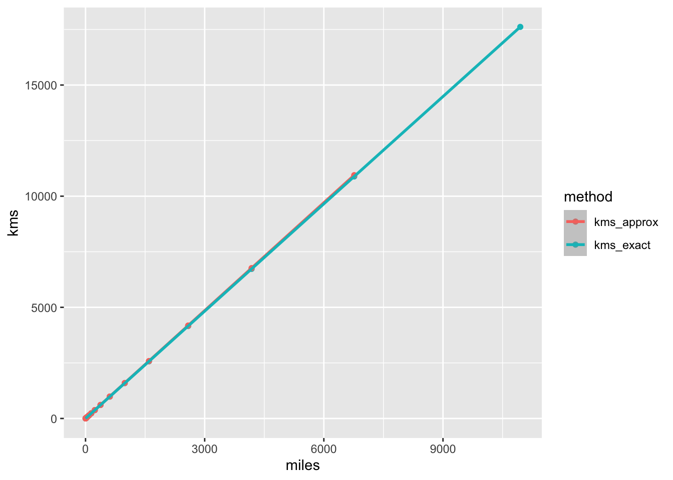
That’s pretty cool. They are so alike that we cant even really see that there are two lines there. The lines are almost exactly over the top of each other.
Lets zoom into the beginning of the plot to see what the differences are like there.
p + facet_zoom(xlim = c(0, 8), ylim = c(0, 25), horizontal = FALSE)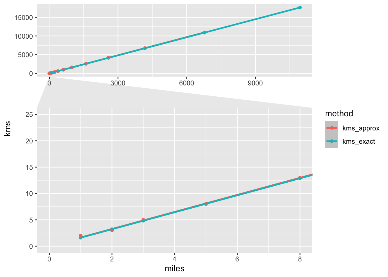
We can now see some differences, but they’re pretty tiny. For an estimation this would be more than enough.
Lets have a look at what the error is per point
df <- df %>%
  mutate(
    kms_diff = kms_exact - kms_approx,
    row = row_number(),
    direction = kms_diff < 0
         )

ggplot(df, aes(x = row, y = kms_diff, fill = direction)) +
  geom_col()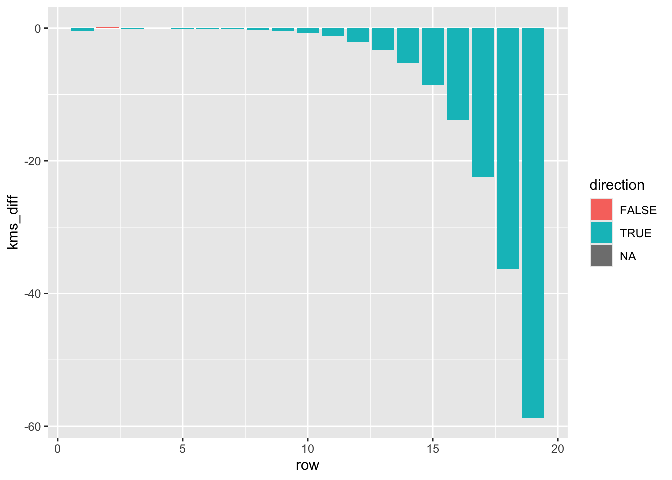
Very interesting. It seems that this method pretty consistently makes the estimation slightly bigger than the exact one. There are only a couple of bars near the beginning where the exact kms were bigger than the approx kms.
I wonder if that trend holds for larger values of n? This will start to get impossible to visualise due to the fibonacci sequence growing exponentially, so lets just count the numbers of true/false values.
fib_numbers <- my_fib(500)
kms_exact <- miles_to_km(fib_numbers)

df_larger <- data.frame(
  miles = fib_numbers,
  kms_exact = miles_to_km(fib_numbers),
  kms_approx = lead(fib_numbers, 1)
) %>%
  mutate(
    kms_diff = kms_exact - kms_approx,
    row = row_number(),
    direction = kms_diff < 0
         ) %>%
  na.omit()

ggplot(df_larger, aes(x = direction, fill = direction)) +
  geom_col(aes(y = direction)) +
  geom_text(aes(label = after_stat(count)), stat = "count", vjust = -0.5)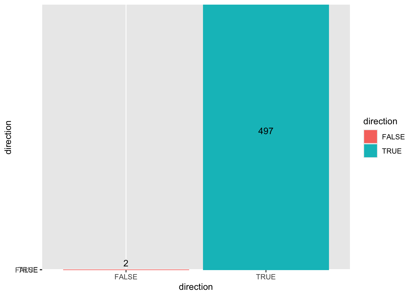
Wow. Calculating out 500 values, and they still maintain the pattern of estimation being slightly bigger than exact.
I’m not a mathematician, so I don’t have a deep understanding of this pattern and why it happens, but regardless, this was a very cool analysis to whip up.
Take care!